Creating Demos - Coder Tutorial #7
[3D Worlds]
By Polaris
Greetings to all you demo coders out there! I hope everyone is healthy and happy,
and enjoying their coding projects!
For this issue I've decided to discuss three dimensional mathematics and how basic "3d"
is achieved. Many people tend to "gloss this over" - because they don't feel that they
need to fully understand it. There are countless postings in forums from people that
are struggling with "gotchas" in Direct X and openGL because they have neglected to master
the basics. Let's master these basics and avoid future struggles!
In this tutorial I'll be teaching you to make wire frame renderings. We'll do the
math ourselves, with basic trigonometry. If you understood my last tutorial,
you are in good shape. If you didn't follow my last tutorial, have a look!
You can also use this refresher on the web: "Trigonometry: A Crash Review".
Check it out here: http://www.zaimoni.com/Trig.htm. As usual, we'll be using Dev C++
and Allegro. Look at older tutorials for refreshers.
With every tutorial, feel free to me questions directly if something doesn't make sense:
Polaris@northerndragons.ca.
Don't forget to tell me what you would like the next tutorial to be. I can't meet
everyone's needs - but I'll certainly try to.
Wireframe Worlds - Cartesian Coordinate Systems (2d)
 The Cartesian Coordinate system was developed by the French mathematician Renť Descartes.
It's rumored that he was sick in bed and was watching a fly buzzing around his ceiling
made of tiles. He didn't have the strength to move to swat it; so he noticed that he
could the count tiles from a specific tile (up/down and left to right) and remember
where the fly was to kill it in the morning. You can imagine pirates doing the same thing
with a land marker. "YAARRGH: From the scull rock, the treasure is 2 paces north, and
5 paces east". The origin is the center of where we start measuring from (in that case
the scull rock).
The Cartesian Coordinate system was developed by the French mathematician Renť Descartes.
It's rumored that he was sick in bed and was watching a fly buzzing around his ceiling
made of tiles. He didn't have the strength to move to swat it; so he noticed that he
could the count tiles from a specific tile (up/down and left to right) and remember
where the fly was to kill it in the morning. You can imagine pirates doing the same thing
with a land marker. "YAARRGH: From the scull rock, the treasure is 2 paces north, and
5 paces east". The origin is the center of where we start measuring from (in that case
the scull rock).
While we don't have evidence that it was a fly that inspired his mathematics - Decartes'
contribution in 1637 was enormous. It's this contribution that all three dimensional
mathematics is based upon, and gave birth to analytic geometry.
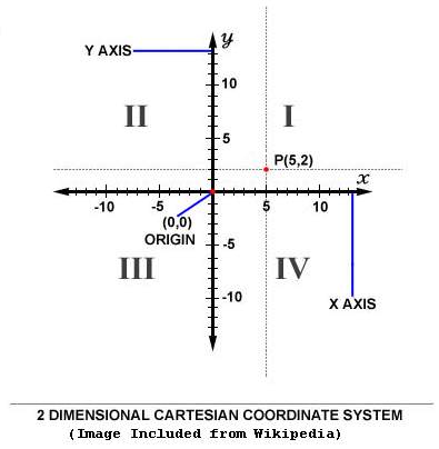
While it should be review for everyone.. here are the basics of the two dimensional
Cartesian coordinate system. The idea is to divide motion into two components.
These are called axes. This is similar to a computer screen - where you have
Screen X (left to right) and Screen Y (up and down). Each axis is like a ruler;
measuring distance along that axis. Every point can be represented by its X value
and Y value. You intersect the two X,Y values - and you know exactly where the point
(or fly) lies. This pair of values is called a coordinate.
The computer screen co-ordinates are setup slightly differently than their
mathematical pure counterpart. In computer graphics the origin at (0,0) is typically
the upper left of the screen, whereas in mathematics - the origin is in the center.
In screen units, as you grow in Y co-ordinates... your Y value goes "down" the screen...
which is exactly opposite to the conventional Y axis in mathematics (upside down).
In the end, this will mean that we'll have to transform our mathematics to the
"screen coordinate system". Usually this is the very last step of any 3d application.
We've already done screen coordinate transformation in the last tutorial on lenses.
Points? It's all about Points? What's the Point????
 So far, I've made a big deal about points. This might seem very trivial, but it's not.
Objects in our three dimensional world - can be represented by points!
So far, I've made a big deal about points. This might seem very trivial, but it's not.
Objects in our three dimensional world - can be represented by points!
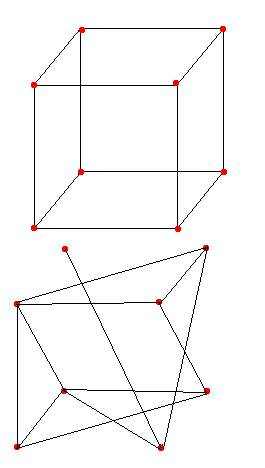
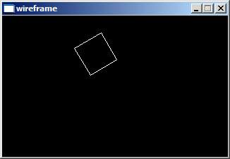
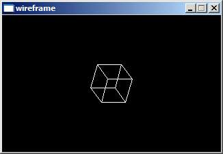
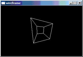
Imagine a cube a moment. A cube has eight outside edges - where its surface comes to
a "point". When we sketch out a cube - we imagine these points connected with lines.
This type of basic rendering is called wire frame (as shown in the picture).
You should realize that we aren't drawing just any lines. Instead we are connecting lines
that are part of the same surface (same shape). In the image, you can see a "cube", as we
normally think about.. and a weird object that shares the same points, but is connected
in an arbitrary way. So, it's not just about points, but putting those points together
as part of a surface.
Any three dimensional surface can be approximated by putting together flat shapes.
This is like Origami (the art of Japanese paper folding). To make a cube, we take
six square shapes and arrange them to form the cube. For a three sided pyramid, we
take 4 triangle shapes (one for the bottom) and arrange them to form a pyramid.
These flat shapes are generically called polygons, and can be any shape (triangle, square,
hexagon). The strictest definition would say - a polygon is a flat shape bounded
by straight lines.
You could render a filled cube (not wire frame) by drawing the six sides (squares) of
the cube and filling them in. This would look similar to old style polygon graphics of
the 1980's. Right now we are doing the same thing, but we aren't bothering to fill our
shapes in. Each of the six sides equates to a single polygon. For now, we'll focus on
just defining wire frame objects and rendering them so they look proper.
We can't represent these points mathematically, unless we have some way to measure them.
This is what coordinates are used for. Later on we can take the coordinates of an object
(like our cube), and rotate them; move them around etc (by using basic math). This is what
enables us to have virtual universes in our computer games and consoles.
Extending into the Third Dimension (Which way is Z?)
Descartes Coordinate system was first envisioned as a two dimensional one.
An easy extension however is to add another measuring stick - the Z axis.
With X,Y, and Z... we can represent any three dimensional point.
These equate to (from a viewer position) - left and right, up and down,
and forward and backward. You can imagine a string hung from Descartes' ceiling,
with markings at the same length as the ceiling tile. This would allow him to
measure how far down the fly was hovering from the ceiling. You would need the
position of the fly in relation to the three axis: X (left, right), Y (up, down),
Z (forward and backward). Our three dimensional origin then becomes (0,0,0).
Oddly enough, mathematics never fully standardized (in my belief) which way "Z"
is measured. If you are holding a coordinate system directly in front of
you, looking towards origin.... does Z increase as you walk forward, or does it
increase as you walk backward? It turns out that this was never fully decided.
Mathematicians found each definition useful in some cases. Instead of forcing
a standard, they came up with two coordinate systems. (Making each a standard.).
The left-handed coordinate system works like this. You take your left hand,
with your palm facing upwards. You point your fingers in the direction of the
positive X axis (to the right). You curl your fingers into the direction of the
positive y-axis (up). Your thumb now points in the direction of the positive Z axis.
This means that Z grows as we "walk forward".
The right-handed coordinate system works almost the same way. You take your
right hand, with your palm facing upwards. Again, you point your fingers
in the direction of the positive X axis (right) and then curl them to the
positive y-axis (up). Your thumb now points in the positive Z axis.
With the right handed system... Z grows as we "walk backward".
To add even more hilarity, computer graphics API's couldn't decide on a
coordinate system (right or left) to be standard either. Open GL uses a
right-handed coordinate system, while Direct X uses a left-handed coordinate system.
I'm going to use the left-handed system for the remainder of the tutorial.
This means that point <0,0,-10> is in front of the origin, while point <0,0,10> is
behind it. I realize this is confusing now, but as we work with it - it should make
more sense.
Transferring to Screen Coordinates (Revisited)
I mentioned above that the computer's origin system starts at the top left
of the screen, at coordinates (0,0). X grows from left to right, which
matches our pure mathematical definition; but Y is upside down (growing as
you go down). We did some screen coordinate conversion in the lens tutorial,
but let's define it here more generally.
The most fundamental thing we need to do is move the origin. The important thing
to remember is that the origin can be anywhere we want it to be. It's the one thing
that's stationary - the "skull rock" that the pirate assumes won't move. We need to
adjust the origin in our math coordinates to be the center of our screen coordinates.
In mode 13h, the center of the screen is (160,100). For us to do this on demand,
we'll use the following equations:
screen_x = pure_x + x_origin_offset
screen_y = -pure_y + y_origin_offset
We'll define our x_origin_offset to have a value of 160 (for mode 13h),
and the y_origin_offset to have a value of 100.
Shapes and Objects - Getting Curvy.
So far we've shown how a cube can be composed from points - which make up surfaces.
In other words, we can build a cube from squares, and squares from points.
You might think that this means that we can only render sharp shaped objects
with our system. How do you make a curve with only points and straight lines?
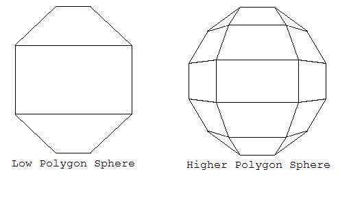
The trick is, that you don't. It's impossible to truly represent a curve with
points connected by straight lines. Instead, we do the best we can by adding
more points and lines to approximate the curve. The more points we add along the
surface of the curve, the better our shape will appear. You can see this with the
shapes that approximate a sphere. In the low polygon sphere, we've only got
3 shapes (or polygons) visible, that give it a "curvy" look. In the higher polygon
sphere, we've added more shapes, points and lines. As we continue to add more polygons,
the sphere becomes more and more defined.
Project #1 - Kicking it 2d
For our first project we'll manipulate a simple two dimensional shape. We'll start with
a square and convert it from pure mathematical co-ordinates to screen coordinates.
After that we'll extend it to perform some basic operations on the points.
Our first project objectives include:
1. Defining a object points.
2. Converting the co-ordinates to screen coordinates.
3. Drawing the object on the screen.
Similar to my last tutorial, we'll start with an basic framework. If you haven't seen
the framework before or are unsure - review the previous articles. You can get
the framework in zip format: wireframe.a.rar in the bonus pack. We will apply our changes to Wireframe.a,
step by step. You'll notice I'm using rar files, which are just like zip files.
To extract them you can download winrar from http://www.rarlab.com/.
1. We'll start by adding our x_origin and y_origin to the code.
I've done this with a pair of #defines, just under our #define's for
sceen_x/screen_y:
#define x_origin_offset 160
#define y_origin_offset 100
2. Following that we need to define a structure to hold our vertices.
We do that just under our #defines:
typedef struct
{
    float x;
    float y;
} Vector2d;
3. At this point we'll add a routine to draw a Wireframe polygon. Let's write the
DrawScreenCords2d routine. It will take a bitmap object (to plot on),
a Vector2d array (what to plot), a colour (how to plot it), and a total # of points
(how many to plot). It will draw a bounded shape of lines for all points.
At the end it will connect the last point to the first point,
a feat achieved using the modulus operator. As screen coordinates are integers,
I've typecast them to integers from floats. (truncating them to screen coordinates).
// converts mathematical points to screen points and plots them.
void DrawScreenCords2d(BITMAP *bitmap,Vector2d *inPoints,int total,int colour)
{
    int i;

    // draw our shape.  Notice this is a closed shape, so point a connects to
    // point b, point b connects to point c, and point c - connects to point a.
    for (i=0;i<total;i++)
    {
    line(bitmap,
        (int)(inPoints[i].x+x_origin_offset),
        (int)(-inPoints[i].y+y_origin_offset),

        (int)(inPoints[(i+1)%total].x+x_origin_offset),
        (int)(-inPoints[(i+1)%total].y+y_origin_offset),
        255);
    }
}
4. Now we need to add our points to the main routine. I've done that right
at the beginning. Notice I'm also adding the variable lOffScreen to hold the
double buffer.
// main constants (more next phase)
Vector2d lSquarePoints[4]=
{
      {20,20}, // top right
      {-20,20},  // top left
      {-20,-20}, // bottom left
      {20,-20} // bottom right
}; // square points
BITMAP *lOffScreen; // off screen buffer
5. Now that we've allocated our points, we need to draw them in our render loop.
We also need to allocate and destroy our off screen render surface. This is added
as follows.
// init more stuff  (next phase)
lOffScreen = create_bitmap(screen_x, screen_y); // NEW

while ((!key[KEY_ESC])&&(!key[KEY_SPACE]))
{
// DO SOMETHING AMAZING HERE!
clear_bitmap(lOffScreen);        //NEW

DrawScreenCords2d(lOffScreen, lSquarePoints,4,255);
blit(lOffScreen, screen, 0, 0, 0, 0, screen_x, screen_y);  // NEW
};

// de-init more stuff  (next phase)
destroy_bitmap(lOffScreen);
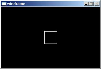
Provided that everything goes according to plan - we should now be able to
compile the code - and enjoy our first Wireframe rendering!
Transformations - Introducing SRT
So far we've been able to create a beautiful square... that does noting
except exhibit perfect square-ness. It would be far more interesting if
we could get our square to do things. There are three fundamental transformations
for all objects - Translation, Scaling and Rotation. (also known as S.R.T).
I'll define each one in turn, show the mathematics used for achieving the effect
and extend our square wireframe program to really dance. We will start with
Translation because it's the simplest transformation.
Translation - The T in SRT
Translating an object - essentially means to move it. If we wanted to move
our square upwards for example, we'd simply add some value to the Y components
of our vertices. Notice I said add, not subtract. Remember that we are dealing
with mathematics at this point and not screen coordinates. Our translation
can also go in the X direction. Because of this, translations are often represented
as a pair of values (for 2d objects), or three values (for 3d objects). Our formula
for translation appears as follows:
new_x = old_x + translation_x
new_y = old_y + translation_y
(and similarly for 3d)
new_z = old_z + translation_z
Let's add translation to our program - step by step:
1. Our first step is to add a translation routine. I've done this just above the
drawing routine.
// At this point I'm doing just floats.  This is because the convert to int
// occurs at the time of drawing.
void Translate2d(Vector2d *inPoints,Vector2d *outPoints,int Total,
                 float xTrans,float yTrans)
{
   int i;

   for (i=0;i<Total;i++)
   {
      outPoints[i].x=inPoints[i].x+xTrans;
      outPoints[i].y=inPoints[i].y+yTrans;
   }
}
2. Now that we have the code to translate our points, we need to make use of it.
The first thing we need to do is introduce some variables:
Vector2d lTranslatedPoints[4]; // translated points
float x_pos;  // object translation
float y_pos;
3. We also need to set our x_pos and y_pos to an intial value. I've done that right
under the create_bitmap used for the off screen buffer.
x_pos=0;
y_pos=0;
4. Our main render loop changes as follows:
while ((!key[KEY_ESC])&&(!key[KEY_SPACE]))
{
   // DO SOMETHING AMAZING HERE!
   clear_bitmap(lOffScreen);

   // adjust SRT's depending on keys
   if (key[KEY_UP])   y_pos++;         // TRANSLATE
   if (key[KEY_DOWN]) y_pos--;
   if (key[KEY_LEFT]) x_pos--;
   if (key[KEY_RIGHT]) x_pos++;

   Translate2d(lSquarePoints,lTranslatedPoints,4,x_pos,y_pos);
   DrawScreenCords2d(lOffScreen, lTranslatedPoints,4,255);
   blit(lOffScreen, screen, 0, 0, 0, 0, screen_x, screen_y);
   rest(10); // prevents it from flying off the screen too FAST
};
5. Voila. Our cursor keys are queried by the if statements, adjusting the y_pos
and x_pos variables. The lSquarePoints are translated by Translate2d, and the
results are stored into lTranslatedPoints.
Scaling - The S in SRT
Scaling an object isn't much different from translating it. With scaling, instead of
moving an object by X,Y or Z values - we stretch (or compress) an object in X,Y,Z
values. We do this with a scaling factor. Scaling an object by 0.5 will shrink
it by a half, scaling by 1.0 will remain the same, and scaling by 2.0 will double
the object. When I say "double / half etc".. I'm referring to the distance
between our vertices. Remember we don't have to scale an object in all three dimensions
simultaneously; it's possible for us to scale our square by different values for
the axis - creating rectangles or other alternate shapes. Scaling is most often thought
of as a general object modifier (changing height, width and breadth simultaneously), and
we'll code it just like that.
new_x = old_x * scale_x
new_y = old_y * scale_y
(and similarly for 3d)
new_z = old_z * scale_z
At this point we'll code our scaling routine. We will also combine it with the
translated values, allowing us to scale and translate our object. Our changes will
look very similar to our translation code, with only a few exceptions.
1. Our first step is to add our scaling routine.
void Scale2d(Vector2d *inPoints,Vector2d *outPoints,int Total,float scale);
{
    int i;

    for (i=0;i<Total;i++)
    {
        outPoints[i].x=inPoints[i].x*scale;
        outPoints[i].y=inPoints[i].y*scale;
    }
}
2. We'll add another set of variables to allow us to scale our points.
To make it clear:
Vector2d lTranslatedPoints[4]; // translated points
BECOMES:
Vector2d lTranslatedAndScaledPoints[4]; // translated and scaled points
and we add:
Vector2d lScaledPoints[4]; // translated points
float scale; // object scale
3. We need to initialize our scale (at the same place that we initialize x_pos and y_pos).
x_pos=0;
y_pos=0;
scale=1; // notice it's one (== no change)
4. Our main render loop changes as follows:
    while ((!key[KEY_ESC])&&(!key[KEY_SPACE]))
    {
        // DO SOMETHING AMAZING HERE!
        clear_bitmap(lOffScreen);

        // adjust SRT's depending on keys
        if (key[KEY_UP])   y_pos++;         // TRANSLATE
        if (key[KEY_DOWN]) y_pos--;
        if (key[KEY_LEFT]) x_pos--;
        if (key[KEY_RIGHT]) x_pos++;

        if (key[KEY_Q]) scale+=0.1;  // scale
        if (key[KEY_A]) scale-=0.1;
        if (scale<0) scale=0;  // prevents scaling with - number

        Scale2d(lSquarePoints,lScaledPoints,4,scale); // scale
        Translate2d(lScaledPoints,lTranslatedAndScaledPoints,4,x_pos,y_pos);
        DrawScreenCords2d(lOffScreen, lTranslatedAndScaledPoints,4,255);
        blit(lOffScreen, screen, 0, 0, 0, 0, screen_x, screen_y);
        rest(10); // prevents it from flying off the screen too FAST
    };
5. Voila! Our q and a keys now scale our object, and our cursor keys now allow us
to translate it.
Rotation - The R in SRT
Rotation is our most difficult transformation. While I'll explain how the
rotation formulas work on the inside, you don't need to understand them to make use of them.
Remember, all we need to do is think in terms of points - lines and surfaces will follow.
To make things even simpler, I'll focus on top down rotations (just like our 2d graphics
here).
Rotations are defined by two fundamental things. The pivot point (where we are rotating),
and the degree of rotation. As we'll need to use trigonometry to calculate our
rotations - our degrees will not be in angles... but instead will be in radians.
Radians are just another unit of measure of angle. Radians are based on the value of PI.
In radians, PI represents a 180 degree rotation. Similarly, 1/2 PI is a 90 degree
rotation. Imagine this to be just the same as exchanging currencies. One currency
is called degrees, and the other is called radians. 180 degrees is roughly 3.14 Radians
(a truncated value of PI).
We can convert between radians and degrees as follows
Radian = (Degree / 360) * 2PI
Degree = (Radian / 2PI) * 360.
(Where 2PI == something like 6.28).
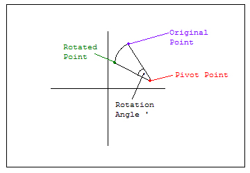
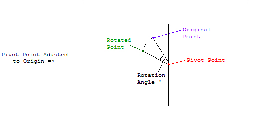
Now, to simplify matters - we are going to develop our formulas with the pivot point
at the origin. This doesn't change our capabilities, if we wanted to develop a rotation
formula to have an arbitrary pivot point, we still can. In that situation we'd use
translation to move the pivot point to our origin, perform the rotation, and then reverse
the translation to move everything back to the pivot point. Since our simplification
doesn't change our capabilities - we'll setup our formulas to pivot around the origin.
Our first rotation formula will be the standard 2d rotation. We will consider each rotation
in terms of axis. To start with, we'll define a Z rotation - which is the standard rotation
for a top down / traditional 2d view. It's like someone glued our object to the Z axis
and then twisted the Z axis by the degrees desired. Our other rotations will be for
the X and Y axes respectively. Let's define our rotation formulas.
Aside: For those familiar with my articles in Hugi - the following definitions
will seem very familiar. They should - because they are identical to my Article in Hugi 27
(Sphere Tessellation 101: "The Art of Making Spheres out of Triangles"). If you are
interested in seeing another application of these formulas (to build spheres etc) - check it
out. Diskmag version: http://hugi.scene.org/fate.php?page=hugi27).
For each rotation around an axis, there are two equations. There isn't a third equation,
as when you rotate around an axis, your value for that axis (x,y,z) does not change.
For example, your Z value for a point will not change if you rotate a point around the
Z axis. Etc.
Here the following formulas:
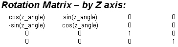
Z Axis Rotation
New_X = x * cos(z_angle) - y * sin(z_angle)
New_Y = y * cos(z_angle) + x * sin(z_angle)
X Axis Rotation
New_Y = y * cos(x_angle) - z * sin(x_angle)
New_Z = y * sin(x_angle) + z * cos(x_angle)
Y Axis Rotation
New_Z = z * cos(y_angle) - x * sin(y_angle)
New_X = z * sin(y_angle) + x * cos(y_angle)
Did you take my word on it? I didn't think so. So, let's look at one of these in detail.
Just realize that all you need is to know how to apply the formulas.
Knowing how it works is just a bonus.
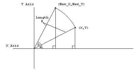
In the diagram, we are rotating point X,Y by angle B. We start however at angle a.
Now, let me introduce some trigonometric identities. [Take my word on these okay?].
cos(a+b) = cos(a)cos(b) - sin(a)sin(b)
sin(a+b) = sin(a)cos(b) + cos(a)sin(b)
Now, our previous point (X,Y) can be expressed as functions of sine and cosine.
Recalling that cosine is the ratio of the adjacent side to the hypotenuse
(or in our case R) we can calculate X as R*cos(a). Sine is the ratio of the
opposite side to the hypotenuse (still R) so we can calculate Y as R*sin(a).
So... X,Y can be represented as:
X = R*cos(a)
Y = R*sin(a)
Now, using this and the identities - we can calculate Z axis functions for a given angle
as follows:
New_X   = R*cos(a+b)
        = R*cos(a)*cos(b) - R*sin(a)*sin(b)  [care of trig identity]
        = X*cos(b) - Y*sin(b) [our formula!]
New_Y   = R*sin(a+b)
        = R*sin(A)*cos(b) + R*cos(a)*sin(b)  [care of trig identity]
        = Y*cos(b) + X*sin(b) [our formula!]
That covers off our rotation formula for Z axis rotations, X and Y axis rotations are
quite similar; so I'm not going to define them here. It's far time that we made something
rotate!
1. Our first step is to add our rotation routine.
void RotateZ2d(Vector2d *inPoints,Vector2d *outPoints,int Total,float ang)
{
    int i;

    for (i=0;i<Total;i++)
    {
        outPoints[i].x = inPoints[i].x * cos(ang) -  inPoints[i].y * sin(ang);
        outPoints[i].y = inPoints[i].y * cos(ang) +  inPoints[i].x * sin(ang);
    }
}
2. We'll add another set of variables to allow us to rotate our points. To make it clear:
We add:
            Vector2d lSRTPoints[4]; // Scaled, Rotated, Translated Points
            float z_angle; // object rotation
3. We need to initialize our rotation (at the same place that we initialize
x_pos and y_pos).
x_pos=0;
y_pos=0;
scale=1;
z_angle=0; // new
4. Our main render loop changes as follows:
    while ((!key[KEY_ESC])&&(!key[KEY_SPACE]))
    {
        // DO SOMETHING AMAZING HERE!
        clear_bitmap(lOffScreen);

        // adjust SRT's depending on keys
        if (key[KEY_UP])   y_pos++;         // TRANSLATE
        if (key[KEY_DOWN]) y_pos--;
        if (key[KEY_LEFT]) x_pos--;
        if (key[KEY_RIGHT]) x_pos++;

        if (key[KEY_Q]) scale+=0.1;  // scale
        if (key[KEY_A]) scale-=0.1;
        if (scale<0) scale=0;  // prevents scaling with - number

        if (key[KEY_W]) z_angle+=0.1;  // rotation
        if (key[KEY_S]) z_angle-=0.1;

        Scale2d(lSquarePoints,lScaledPoints,4,scale); // scale
        Translate2d(lScaledPoints,lTranslatedAndScaledPoints,4, //translate
                x_pos,y_pos);
        RotateZ2d(lTranslatedAndScaledPoints,lSRTPoints,4,z_angle);

        DrawScreenCords2d(lOffScreen, lSRTPoints,4,255);
        blit(lOffScreen, screen, 0, 0, 0, 0, screen_x, screen_y);
        rest(10); // prevents it from flying off the screen too FAST
    };
5. Voila! Our w and s keys now rotate our object.
Run the program and see how it behaves. You might be surprised.....
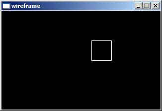
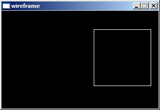
Thou Shalt Pay Attention to the Order of Things (Or Get Weird Results)
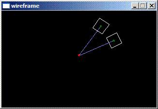
The rotating square might surprise you when you run it. I've shown two cubes
in the picture to illustrate what's happening. The problem is that our algorithms are doing
exactly what we've told them... specifically:
1. Scale our Object
2. Translate our Object
3. Rotate our Object
Because we translated our object - our object is no longer centered on the origin.
Our rotation works fine (kind of orbital)... but probably isn't what a user of the program
would expect. Instead... we'd normally expect our object to rotate at its center.
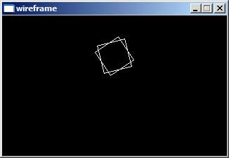
Let's rework the program to do a true SRT:
1. Scale
2. Rotate
3. Translate
Step by step:
1. To prevent confusion, I suggest we change our global variables. In specific:
Vector2d lTranslatedAndScaledPoints[4]; // translated and scaled points
Becomes:
Vector2d lScaledAndRotatedPoints[4]; // Scaled and rotated
2. Our main loop changes slightly... specifically:
Scale2d(lSquarePoints,lScaledPoints,4,scale);
RotateZ2d(lScaledPoints,lScaledAndRotatedPoints,4,z_angle);
Translate2d(lScaledAndRotatedPoints,lSRTPoints,4, x_pos,y_pos);
3. Voila! Now we've got our cube rotating as we'd expect.
You'll notice that the picture shows that our rotation - is now in the center of the object.
Entering the Third Dimension - Perspective and Orthogonal Views "AKA - What to do with Z?".
At this point we are on the cusp of taking things into the third dimension.
We have the math, and the routines to do the graphics; but one question lingers.
"What do we do with Z?" At this point in time, we don't have many three dimensional
displays on the market. So, in truth... three dimensional graphics are never actually
three dimensional. They become flattened by the screen they are projected on.
We need to find a technique to "squish" our mathematics into our flat screen.
The act of squishing our three dimensional object is like creating a projection
of the object. There are two common projection techniques.
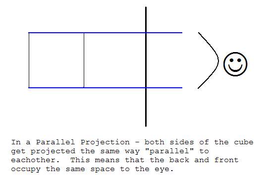
1. Parallel Projection:
A Parallel Projection is the simplest projection. Essentially we drop the Z out
of the system all together. This will be our first projection project. The problem
with a parallel projection is that it doesn't care about how far back our objects are.
If a object is 40 units wide, it will take 40 units on the screen no matter how far from
the virtual viewer it lies.
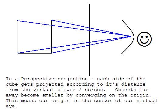
2. Perspective Projection:
A perspective projection is a little more sophisticated. It takes into account or depth
from virtual viewer (situated at the origin), and results in a perspective. This is the
same technique that artists use when painting and sketching. This will be our
second project.
For better understanding, consult the pictures that show a Y / Z oriented view.
The face is looking down the Z axis, centered around the origin. The black line
represents the computer screen - and the curved line shows light being caught by
our virtual eye.
Let's Get Some Three Dimensions!
At this point, we need to extend our square to be a cube - and draw it to the screen.
The simplest thing to do is go back to our wireframe.a.rar, and build our 3d project
from basic principles. We are going to take a basic cube - and allow it to be rotated
with the cursor keys. We'll just do X,Y rotations to illustrate the concepts.
1. We'll start by adding our x_origin and y_origin to the code. I've done this with a
pair of #defines, just under our #define's for sceen_x/screen_y:
#define x_origin_offset 160
#define y_origin_offset 100
2. Our next step is to extend our structure to allow for three dimensional objects.
typedef struct
{
    float x;
    float y;
    float z;
} Vector3d;
3. At this point we need two rotation functions - one for X, the other for Y.
These follow our mathematical formulas:
void Rotate3d_Xaxis(Vector3d *inPoints,Vector3d *outPoints,
                    int Total, float angleRadians)
{
    int i;

    for (i=0;i<Total;i++)
    {
        // X is untransformed, just recopied.
        outPoints[i].x = inPoints[i].x;
        outPoints[i].y = inPoints[i].y * cos(angleRadians)
                          - inPoints[i].z * sin(angleRadians);
        outPoints[i].z = inPoints[i].y * sin(angleRadians)
                          + inPoints[i].z * cos(angleRadians);
    }
}

void Rotate3d_Yaxis(Vector3d *inPoints,Vector3d *outPoints,
                    int Total, float angleRadians)
{
    int i;

    for (i=0;i<Total;i++)
    {
        outPoints[i].x = inPoints[i].z * sin(angleRadians)
                          + inPoints[i].x * cos(angleRadians);
        // Y is untransformed, just recopied.
        outPoints[i].y = inPoints[i].y;
        outPoints[i].z = inPoints[i].z * cos(angleRadians)
                          - inPoints[i].x * sin(angleRadians);
    }
}
4. Our Draw points routine also changes:
void DrawScreenCords3dParallel(BITMAP *bitmap,Vector3d *inPoints,
                               int total, int colour)
{
    int i;

    // draw our shape.  Notice this is a closed
    // shape, so point a connects to point b,
    // point b connects to point c, and
    // point c - connects to point a.
    for (i=0;i<total;i++)
    {
    line(bitmap,
        (int)(inPoints[i].x+x_origin_offset),
              (int)(-inPoints[i].y+y_origin_offset),
        (int)(inPoints[(i+1)%total].x+x_origin_offset),
              (int)(-inPoints[(i+1)%total].y+y_origin_offset),
        255);
    }
}
5. We now need to define our cube. It's like a square - but with a lot more points.
You'll notice I'm keeping things simple for our drawing routine and repeating points
for every surface. That means points 0-3 form one surface, 4-7 form the next,
8-11 form the third... etc. This recopies a lot of points (which isn't good),
but is sufficient for showing how things work.
// main constants (more next phase)
    Vector3d lCubePoints[24]=
    {
        {20,20,-20}, {-20,20,-20},{-20,-20,-20},{20,-20,-20}, // font face
        {20,20,20}, {-20,20,20}, {-20,-20,20},{20,-20,20}, // back face
        {20,20,20}, {20,20,-20}, {-20,20,-20}, {-20,20,20},// top face
        {20,-20,20}, {20,-20,-20}, {-20,-20,-20}, {-20,-20,20}, // bottom face
        {-20,20,20}, {-20,20,-20}, {-20,-20,-20}, {-20,-20,20},  // left face
        {20,20,20}, {20,20,-20}, {20,-20,-20}, {20,-20,20} // right face
    }; // cube Points

    Vector3d lRotatedPointsX[24]; // rotated cube by X axis
    Vector3d lRotatedPointsXY[24]; // rotated cube by X and Y axis
6. We need to add variables to hold our angles. These will be to measure X axis
rotations and Y axis rotations.
float x_angle; // object rotation REMEMBER IN (RADIANS)
float y_angle; // object rotation
7. We also need to initialize these variables:
x_angle=0;
y_angle=0;
8. Last but not least - our main render loop becomes:
    while ((!key[KEY_ESC])&&(!key[KEY_SPACE]))
    {
        // DO SOMETHING AMAZING HERE!
        clear_bitmap(lOffScreen);

        // adjust SRT's depending on keys
        if (key[KEY_UP])    x_angle+=0.5;
        if (key[KEY_DOWN])  x_angle-=0.5;
        if (key[KEY_LEFT])  y_angle+=0.5;
        if (key[KEY_RIGHT]) y_angle-=0.5;

        Rotate3d_Xaxis(lCubePoints,lRotatedPointsX,24,x_angle);
        Rotate3d_Yaxis(lRotatedPointsX,lRotatedPointsXY,24,y_angle);

        for (int i=0;i<24;i+=4)
           DrawScreenCords3dParallel(lOffScreen, &lRotatedPointsXY[i],4,255);

        blit(lOffScreen, screen, 0, 0, 0, 0, screen_x, screen_y);
        rest(10); // prevents it from flying off the screen too FAST
    };
9. Voila! That took a few more steps, but you can now enjoy a rotating 3d cube.
You'll notice that the drawing loop is set up to draw surfaces of four vertices each.
If you need to catch up or compare, download wireframe.g.rar.
Let's Get Some Perspective
 While it's finally great to see a rotating cube; when you first start the program
with no rotation - all you will see is a square. That's because the first surface
is identical to the second surface in a parallel projection. Now we need to compensate
by adjusting the size of objects that are far away. We do this by centering our world
against the origin. We shrink things that are far away; keeping things nearby unaffected.
Our newly adjusted far away points "converge" on the origin, giving the view perspective.
It's not nearly as hard as it looks.
While it's finally great to see a rotating cube; when you first start the program
with no rotation - all you will see is a square. That's because the first surface
is identical to the second surface in a parallel projection. Now we need to compensate
by adjusting the size of objects that are far away. We do this by centering our world
against the origin. We shrink things that are far away; keeping things nearby unaffected.
Our newly adjusted far away points "converge" on the origin, giving the view perspective.
It's not nearly as hard as it looks.
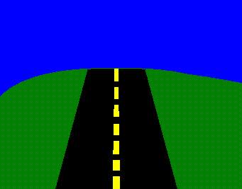
Imagine how a car simulator works... the road directly ahead looks larger than the road
behind. That's because the road ahead is larger - taking more screen space... then the
road at the end of the horizon. This is the perspective effect we are going to achieve.
The simplest way to achieve the effect is to adjust our X and Y according to the
Z distance. This simply looks like:
Perspective_X = Vertex X / Vertex Z
Perspective_Y = Vertex Y / Vertex Z
Now, this does make some assumptions about our coordinate system. It means that we
are looking from the origin, and that all our world is in +Z values, or is culled
off screen. If we imagined our virtual viewer to be outside the origin (Ie, in -Z),
our geometry would not only flip (upside down), but it would also scale nearby objects
smaller. To avoid this we will assume our geometry is actually in +Z values before
we flip to a perspective view. We aren't quite ready yet however, as we don't yet
know how "deep" our screen should be. If we divide by Z, it's quite possible that
our object will simply shrink away to nothingness.
We get around this by extending our formulas:
Perspective_X = fScale*Vertex X / Vertex Z
Perspective_Y = fScale*Vertex Y / Vertex Z
fScale simply defines how the Z affects our view. Consider like a lens factor.
At this point - we are ready to begin our implementation.
1. First of all - we need to define fScale.
#define fScale 40
2. Since we need to make sure our object exists in positive Z axis,
we push it "back" by translation. Hence we need a translation function,
at least for Z. Here is a generic one.
void Translate3d_XYZ(Vector3d *inPoints,Vector3d *outPoints,int Total,
                     float x,float y,float z)
{
    int i;

    for (i=0;i<Total;i++)
    {
        outPoints[i].x = inPoints[i].x+x;
        outPoints[i].y = inPoints[i].y+y;
        outPoints[i].z = inPoints[i].z+z;
    }
}
3. We need a place to store our translated points... so we add new variable.
Vector3d lRotatedPointsXY_Translated[24]; // rotated then translated
4. Our last transformation is to push the object backwards, and call our
new drawing routine (which we will soon write):
// Translate the object 40 units forward to force Z into positive units
Translate3d_XYZ(lRotatedPointsXY,lRotatedPointsXY_Translated,24,0,0,40);

for (int i=0;i<24;i+=4)
DrawScreenCords3dPerspective(lOffScreen, &lRotatedPointsXY_Translated[i],4,255);
5. And now - we need to add our drawing routine, which looks like our formulas:
// converts mathematical ponts to screen points and plots them. (PERSPECTIVE)
void DrawScreenCords3dPerspective(BITMAP *bitmap,Vector3d *inPoints,int total,
        int colour)
{
    int i;

    // draw our shape.  Notice this is a closed shape, so point a connects to
    // point b, point b connects to point c, and point c - connects to point a.
    for (i=0;i<total;i++)
    {
    line(bitmap,
        (int)(fScale*inPoints[i].x/inPoints[i].z+x_origin_offset),
        (int)(fScale*-inPoints[i].y/inPoints[i].z+y_origin_offset),
        (int)(fScale*inPoints[(i+1)%total].x/inPoints[(i+1)%total].z
              +x_origin_offset),
        (int)(fScale*-inPoints[(i+1)%total].y/inPoints[(i+1)%total].z
              +y_origin_offset),255);
    }
}
6. Voila! We now have a rotating cube with perspective. It looks a bit odd
from time to time - but mostly that's relating to the view scale etc... feel free
to adjust the cube size / fScale to get things right for your application.
Object Hierarchies
At this point we've exposed all the mathematics required to do basic Wireframe graphics.
There obviously is quite a difference between a cube and a complicated object however - and
I want to discuss some of that now. Objects are rarely in isolation. Animating a
simple car would require moving both the wheels - and the frame of the car.
Animating a helicopter is the same idea - the rotor moves around; but it's attached
to the cockpit. Usually we create a chain of SRT transformations to adjust objects
from being in "object space" or "model space", to their final position in world space.
In a simple example:
1. We rotate the rotor of a helicopter (rotation along the Y axis). The rotor is centered around the origin.
2. We translate the rotor upwards (according to the height of the cockpit). This means the object can be rendered along side the cockpit and it will "match".
3. We perform any SRT to both the adjusted (rotated / and translated) rotor, as well as the cockpit. This allows us to place the completed helicopter anywhere we want into three dimensional space.
The concepts for a simple helicopter extend to all objects that have relationships.
These types of spatial relationships are known as an object hierarchy. The most useful
area to use an object hierarchy is in character animation. You might start at the torso,
add an upper arm, add a fore arm, add a hand (with wrist), add each finger - each with
3 segments. Once we get to render the end of the finger - we will have passed through
six joints - and possibly six unique SRT transformations. We need to consider both
the orientation of the joint, as well as how and where the bone will connect.
The problem however - is that at a certain point we get overwhelmed by all
our transformations. Wouldn't it be nicer if there was an intelligent way to group
a series of transformations - into a single unit? There is a better way...
called Matrices.
Enter the Matrix!
The ultimate goal of any real time computer graphics is to render to the screen
as quickly as possible. While we've defined our transformations, it's easy for them
to get unruly, in both complexity and calculation time. Matrices give us a way
to reduce the number of calculations performed - while simplifying our work, and improving
calculation speed. It's possible to have a single matrix represent a X translation,
a Y translation, a Z translation, Scaling X, Scaling Y, Scaling Z, Rotation in X, Rotation
in Y and Rotation in Z!!! Talk about one stop shopping!
It gets even better. Not only can we represent a series of transformations into
a matrix - but we can also perform operations on matrices. So, if we have a matrix
that performs a Scaling, but we also want to do rotations - we can combine these
two matrices using Matrix Arithmetic. We get a new matrix which does not only
the scaling but also the rotation. Computers equipped with MMX or SIMD type systems
are especially suited for matrix applications. Direct X includes a library of
matrix functions in D3DX - which are optimized to work very efficiently on any cpu.
However, for now we'll code them ourselves to get you used to the idea of matrices.
Show me the Matrix!
Matrices are a generic concept in mathematics, and matrix is just another word
for a table of numbers. Matrices can be any size - and shape (they don't have to
be a flat table either). Computer graphics use a simple matrix (only 4 rows by 4 columns),
for a total of 16 values. A simple matrix for computer graphics could appear as follows:
 1   2   3   4
 5   6   7   8
 9  10  11  12
13  14  15  16
Remember that matrices aren't limited to being square or 4x4. It's just as possible
to have a matrix with just one row. A set of 3d points (x,y,z) - could be stored
in a 1x3 matrix. A 1x3 matrix is also called a vector, which is very useful because
it's a "point" in our three dimensional space. Now, assuming that we have a matrix
(grid of numbers) and a vector... how do we find out our new x,y,z? We use matrix
multiplication to calculate a new vector.
New VectorX,Y,Z = Old Vector X,Y,Z * Matrix
Please realize that this isn't your standard multiplication that you learned in
grade school. This is matrix multiplication, which defines the shape of the
resulting matrix (how many columns and rows), and how to map between your two
input matrices and create a resulting matrix. It's not nearly as complicated as
it sounds. It turns out that when matrix multiplication was defined, it was defined
with a restriction. You can only multiply matrices if the number of columns of the
first matrix is the same as the number of rows of the second matrix. Do you notice
a problem?
I've told you that you can represent SRT transformations in a 4x4 matrix,
but we need to use matrix multiplication to calculate the results of a 3 element vector.
A three element vector only has 3 columns, which is one shy of the required 4 columns.
How do we get around this? Easy - we use the simplest trick in the book and
fudge the numbers. To get our resulting transformation, we add an extra element.
New Vector <X,Y,Z, ignored> = Old Vector <x,y,z,ignored> * Matrix.
We'll set the ignored value to one so it doesn't affect our calculations.
It will be used in the matrix calculations - but ultimately thrown away.
We can craft specific vector instructions to drop them out at the start - but either way..
they don't get used.
So, what does matrix multiplication look like? Let's say we are multiplying two
matrices - A and B. We know that A has the same number of columns - as the number
of rows of B. This is essential to our mapping. We map the columns of A - to the rows
in B.
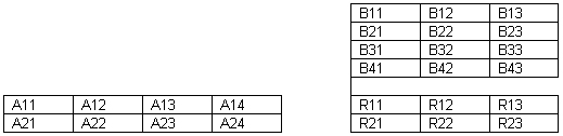
Here I've plotted two matrices. A is a 2x4 matrix. B is a 4 by 3 matrix.
The number of columns in A is 4, and the number of rows in B is also 4.
So we know we can multiply these two matrices. I've put boxes around the matrices so
you can tell which belong together.
I've labeled the entries in our matrix as A?* - where ? is the row, and * is the column.
Similarly, I've done the same with Matrix B, and Matrix R - our resulting matrix.
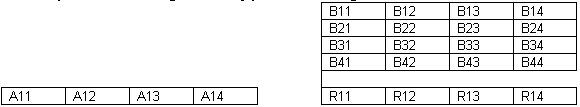
If Matrix A is a MxN matrix (M rows by N columns) and Matrix B is a NxP matrix
(N rows by P columns) we get a MxP matrix. IE, Matrix R will have the same number
of rows as Matrix A, and the same number of columns as matrix B.
To calculate our result, we multiply according to the intersection of rows and columns
in A and B. For example: R11 is the result of multiplying matrix A's first row, and
Matrix B's first column. R21 is the result of multiplying the second row of Matrix A
and the First row of Matrix B. It's like looking up the timetable of the bus.
Every square in the result section, depends on the matrix A values on its left, and
the Matrix B values on the right. We still haven't said how it depends - but that's
the easy part.
Each R is calculated as the sum of A values multiplied by B values. For example:
R22 = A21*B12 + A22 * B22 + A32 * B32 + A23 * B42
You can trace your fingers along this path. You start with A21, and B12.
These two multiply. We then move on to the next square, A22 and B22.
These multiply and are added to our series. So on and so forth - until we've done
the calculation. We can easily write some for loops to do this transformation.
Mathematically it's expressed in summation notation which this looks like the following:
To solidify our understanding, let's multiply a 1x4 vector against a 4x4 matrix
R11 = A11*B11 + A12*B21 + A13*B31 + A14*B41
R12 = A11*B12 + A12*B22 + A13*B32 + A14*B42
R13 = A11*B13 + A12*B23 + A13*B33 + A14*B43
R14 = A11*B14 + A12*B24 + A13*B34 + A14*B44
That gives us our mathematics to express our vector * matrix multiplication.
Let's express the same thing in code. Vector is our inbound vector (integer [4]),
our result vector is called result (integer[4]), and matrix is our transformation matrix
(integer[4][4]). The code unrolled looks as follows:
result[0]=vector[0]*matrix[0][0] + vector[1]*matrix[1][0] + vector[2]*matrix[2][0] + vector[3]*matrix[3][0];
result[1]=vector[1]*matrix[0][1] + vector[1]*matrix[1][1] + vector[2]*matrix[2][1] + vector[3]*matrix[3][1];
result[2]=vector[2]*matrix[0][2] + vector[1]*matrix[1][2] + vector[2]*matrix[2][2] + vector[3]*matrix[3][2];
result[3]=vector[3]*matrix[0][3] + vector[1]*matrix[1][3] + vector[2]*matrix[2][3] + vector[3]*matrix[3][3];
We can of course roll this up - it looks a bit neater like this
(but isn't quite as fast because of the for loop taking some extra code):
int i;
for (i=0;i<4;i++)
{
   result[i]=vector[i]*matrix[0][i] + vector[1]*matrix[1][i]
             + vector[2]*matrix[2][i] + vector[3]*matrix[3][i];
}
We can role it up even further - but I think you get the idea. In review so far - we've
shown that points <x,y,z> can be expressed as a 1x4 matrix. We've illustrated that
matrices can be multiplied by vectors to transform the vector. We can scale a vector
by multiplying it by a scaling Matrix. We can rotate vectors by rotating it by a
rotating matrix. I haven't yet shown what those matrices look like - that's the next
step. The one thing I want you to learn is this: We don't just use matrix multiplication
(also called concatenation) to calculate the result of vectors transformed by a matrix.
We use it to multiply matrices together.... concatenating matrices.
For example:
Matrix A == Scaling Matrix
Matrix B == Rotating Matrix
Matrix C == Matrix A * Matrix B == A matrix that scales and then rotates.
In code, the concatenation of two 4x4 matrices appears as follows:
(just one implementation)
C=A*B
for (int i=0; i<4; i++)
   for (int j=0; j<4; j++)
   {
      C[i][j]=0; // init output matrix

      for (int k; k<4; k++)
         C[i][j]+=A[k][j]*B[k][j];
   }
It's generic matrix multiplication that allows us to combine all our crazy transformations
into a single matrix package. That's what all this fuss (and work) is about.
SRT Matrices
It's high time now that we looked at the transformation matrices that we can use to
apply SRT - scaling, rotation and translation. Remember all of these are 4x4 Matrices,
and when multiplied by a 1x4 vector result in the operation being performed against that
vector. The matrices can be combined to create a "combined transformation matrix".
Let's define all our SRT matrices:
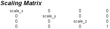
Scales by scale_x, scale_y, scale_z. Notice if scale_x=1, scale_y=1, and scale_z=1 we
get a matrix that doesn't affect the geometry. This is called an identity matrix,
as any matrix * Identity = the same matrix. Identity matrices can be easily recognized
as they have zero for all values except the diagonal - (top left to bottom right) which is
set to one.
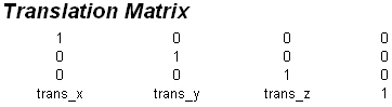
This translates our vector by trans_x, trans_y, and trans_z. You might notice that we
could easily add scaling too - by replacing the first few 1's (diagonal) with
scale_x, scale_y, and scale_z. Just remember, that as we re-use cells in our matrix
it can be more difficult to overlaying another matrix to combine them. To combine matrices
into a single transformation - multiply them out! (Concatenate them!)
Implementing - The Matrix
Our last project will be to implement some matrix arithmetic into the works.
Ideal in terms of operations (and simplifying the math), we'd collect up our
transformations and multiply them out. This will create a new matrix that we'll use
to transform the object any way we please. In practice, the computer is fast at
multiplying out matrices (using SIMD type operations)... and usually transformations
are composed using the graphics api rather than manually working them out. We'll
do that here too - so we can easily flow into that model of doing things later.
(I want you to understand the nuances of using matrices, you can optimize the hell
out of it later.)
Our first step will be to introduce some new functions: Specifically, functions to
multiply matrices, vectors, and do rotation and translations.
/*----------------------------------------------------------------------------*/
// mat R == result matrix
void MultiplyMatrix(float matR[4][4], float matA[4][4], float matB[4][4])
{ // no optimizations here
for (int i=0;i<4;i++)
{
for (int j=0;j<4;j++)
{
matR[i][j]=0;
for (int k=0;k<4;k++)
{
matR[i][j]+=matA[i][k]*matB[k][j];
}
}
}
}
/*----------------------------------------------------------------------------*/
void MultiplyVectors(Vector3d *inPoints,Vector3d *outPoints,int Total,
float mat[4][4])
{
int i;
// somewhat streamlined matrix * vect function
for (i=0;i<Total;i++)
{
// copy result out.
outPoints[i].x=
inPoints[i].x*mat[0][0] +
inPoints[i].y*mat[1][0] +
inPoints[i].z*mat[2][0] +
mat[3][0]; // (1 fudge)
outPoints[i].y=
inPoints[i].x*mat[0][1] +
inPoints[i].y*mat[1][1] +
inPoints[i].z*mat[2][1] +
mat[3][1]; // 1 fudge
outPoints[i].z=
inPoints[i].x*mat[0][2] +
inPoints[i].y*mat[1][2] +
inPoints[i].z*mat[2][2] +
mat[3][2]; // 1 fudge
}
}
/*----------------------------------------------------------------------------*/
// creates a translation matrix for x,y,z translation
void TranslationMatrix(float matR[4][4],float x,float y,float z)
{
// clear matrix;
int i,j;
for (i=0;i<4;i++)
for (j=0;j<4;j++)
{
if (i==j)
matR[i][j]=1;
else
matR[i][j]=0;
}
// at this point we have an identity matrix
// fill in the other values
matR[3][0]=x;
matR[3][1]=y;
matR[3][2]=z;
}
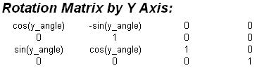
/*----------------------------------------------------------------------------*/
void RotateYMatrix(float matR[4][4],float y_angle)
{
// clear matrix;
int i,j;
for (i=0;i<4;i++)
for (j=0;j<4;j++)
{
if (i==j)
matR[i][j]=1;
else
matR[i][j]=0;
}
// at this point we have an identity matrix
// fill in the other values
matR[0][0]= cos(y_angle);
matR[0][2]= -sin(y_angle);
matR[2][0]= sin(y_angle);
matR[2][2]= cos(y_angle);
}
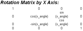
/*----------------------------------------------------------------------------*/
void RotateXMatrix(float matR[4][4],float x_angle)
{
// clear matrix;
int i,j;
for (i=0;i<4;i++)
for (j=0;j<4;j++)
{
if (i==j)
matR[i][j]=1;
else
matR[i][j]=0;
}
// at this point we have an identity matrix
// fill in the other values
matR[1][1]= cos(x_angle);
matR[1][2]= sin(x_angle);
matR[2][1]= -sin(x_angle);
matR[2][2]= cos(x_angle);
}
Our main program changes now... to use mostly matrices instead of vector lists.
These include:
    float XrotMat[4][4];     // X rotation Matrix
    float YrotMat[4][4];     // Y rotation Matrix
    float TransMat[4][4];    // translation Matrix
    float XYRotMat[4][4];    // X rotation, Y rotation
    float World[4][4];       // X,Y rotation + Translation
                             // (combined into a world matrix)
    Vector3d renderPoints[24]; // points to render
The guts of our render loop also change:
       // compose our X rotation and Y rotation matrices
        RotateXMatrix(XrotMat,x_angle);
        RotateYMatrix(YrotMat,y_angle);

        // Set up Translation matrix (notice since it's constant we don't
        // need to calc!)
        TranslationMatrix(TransMat,0,0,40);

        MultiplyMatrix(XYRotMat,XrotMat,YrotMat);
        MultiplyMatrix(World,XYRotMat,TransMat); // rotate , then translate

        // multiply our points
        MultiplyVectors(lCubePoints,renderPoints,24,World);
        for (int i=0;i<24;i+=4)
                DrawScreenCords3dPerspective(lOffScreen, &renderPoints[i],4,255);
Voila! You are now rendering with matrices. This is less efficient in our
contrived example of only a cube, but on the whole in a large examples this will be
more efficient. If you got lost along the way - catch up with wireframe.i.rar.
The end of the Matrix?
Well, not exactly. We've only scratched the surface of what's available.
Later on we'll dig into Direct X and/or Open GL -> and we'll use the d3dx functions
to do our matrix math. However, having coded and mastered this - you've got an
unbeatable understanding of matrices.
For those wishing to pursue further - do some searching for "matrix stacks".
They are very useful for object hierarchies, and are built into Open GL (natively),
and direct x (as part of the d3dx library).
In addition for an extra challenge - you might examine ways to prevent from
duplicating vertices. There are two things to look for about this:
1. Triangle fans and strips (a way of representing a shape while reducing the number
of duplicated vertices).
2. Vertex indexing ;-).
Coming Soon!
Well folks, as promised - I respond to reader requests. I haven't decided what's
next..... but I'm already looking forward to it.
Will it be a:
1. Extension on our Wireframe graphics?
2. Scrollers 201? Working towards a scroller generation program?
3. Or something completely different?
Don't forget to cast your vote and email me at: polaris@northerndragons.ca.
In the mean time - take care!
Polaris